Watching the NFL preseason is always a paradox. Last week as the Seahawks closed out game 4 against the Raiders, I was simultaneously glued to the TV and telling myself the game was totally meaningless.
The general wisdom of preseason play is that while it helps teams prepare and figure out how to sort players for the final depth chart, the outcomes of the games don’t have any bearing on the regular season. To put this theory to the test, I went to the data.
I used the awesome nflscrapR package to pull the results of all preseason and regular season NFL games from 2009 through 2018.
#devtools::install_github(repo = 'maksimhorowitz/nflscrapR')
library(png)
library(grid)
library(furrr)
library(scales)
library(ggrepel)
library(ggridges)
library(tidyverse)
library(nflscrapR)
plan(multiprocess)

years <- 2009:2018

calc_season_data <- function(year) {
    reg_games <- scrape_game_ids(year, type = 'reg')
    preseason_games <- scrape_game_ids(year, type = 'pre', weeks = 1:4)
    rbind(reg_games, preseason_games)
}
Note this next step can take almost an hour to run, so to speed up the process I used furrr to run through the years in parallel.
all_game_data <- future_map_dfr(years, calc_season_data, .progress = TRUE)head(all_game_data)## type game_id home_team away_team week season state_of_game
## 1 reg 2009091000 PIT TEN 1 2009 POST
## 2 reg 2009091304 CLE MIN 1 2009 POST
## 3 reg 2009091307 NO DET 1 2009 POST
## 4 reg 2009091308 TB DAL 1 2009 POST
## 5 reg 2009091305 HOU NYJ 1 2009 POST
## 6 reg 2009091306 IND JAC 1 2009 POST
## game_url
## 1 http://www.nfl.com/liveupdate/game-center/2009091000/2009091000_gtd.json
## 2 http://www.nfl.com/liveupdate/game-center/2009091304/2009091304_gtd.json
## 3 http://www.nfl.com/liveupdate/game-center/2009091307/2009091307_gtd.json
## 4 http://www.nfl.com/liveupdate/game-center/2009091308/2009091308_gtd.json
## 5 http://www.nfl.com/liveupdate/game-center/2009091305/2009091305_gtd.json
## 6 http://www.nfl.com/liveupdate/game-center/2009091306/2009091306_gtd.json
## home_score away_score
## 1 13 10
## 2 20 34
## 3 45 27
## 4 21 34
## 5 7 24
## 6 14 12To prepare the data for analysis, I calculated each team’s cumulative winning percentage for all ten seasons, filtering out ties.
results_df <- all_game_data %>%
    mutate(winner = case_when(home_score > away_score ~ home_team,
                              away_score > home_score ~ away_team),
           loser = case_when(home_score > away_score ~ away_team,
                             away_score > home_score ~ home_team)) %>%
    count(season, type, winner, loser) %>%
    gather(outcome, team, c(winner, loser)) %>%
    group_by(team, season, type) %>%
    summarise(wins = sum(n[outcome == 'winner']),
              games = n()) %>%
    ungroup() %>%
    filter(!is.na(team)) %>%
    group_by(team, type) %>%
    summarise(pct = sum(wins) / sum(games)) %>%
    ungroup() %>%
    spread(type, pct) %>%
    arrange(-reg)

head(results_df)
## # A tibble: 6 x 3
## team pre reg
## <chr> <dbl> <dbl>
## 1 NE 0.55 0.860
## 2 LAC 0.375 0.724
## 3 PIT 0.525 0.720
## 4 GB 0.6 0.709
## 5 NO 0.475 0.690
## 6 LA 0.5 0.651To look for a correlation, I plotted the preseason versus regular season winning percentages for each team.
results_df %>%
    mutate(color = case_when(
        team == 'NE' ~ 'blue',
        team == 'CLE' ~ 'brown',
        TRUE ~ 'black'
    )) %>%
    ggplot(aes(x = pre, y = reg)) +
    geom_point() +
    theme_minimal() +
    scale_x_continuous(labels = function(x) percent(x, accuracy = 1)) +
    scale_y_continuous(labels = function(x) percent(x, accuracy = 1)) +
    labs(x = 'Preseason winning percentage',
         y = 'Regular season winning percentage',
         title = 'The NFL preaseason isn\'t predictive of the regular season',
         subtitle = 'Each dot represents a team\'s cumulative record from 2009-2018') +
    geom_text_repel(aes(label = team, color = color)) +
    scale_color_manual(values = c('brown' = 'brown', 'blue' = 'blue', 'black' = 'grey')) +
    theme(legend.position = 'none')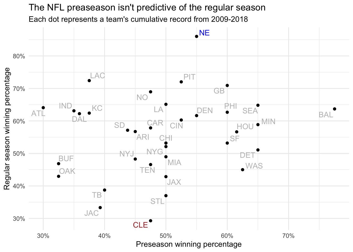
This chart supports the consensus view that the preseason doesn’t provide any insight into a team’s regular season performance. There’s no visible correlation between preseason and regular season wins, and the best and worst teams are nearly identical in terms of preseason play. The Patriots, who boast an 86% regular season winning percentage over the past 10 years, are barely above 50% in the preseason. The Browns, meanwhile, have been only slightly less successful in the preseason but have won fewer than 30% of their regular season matchups.
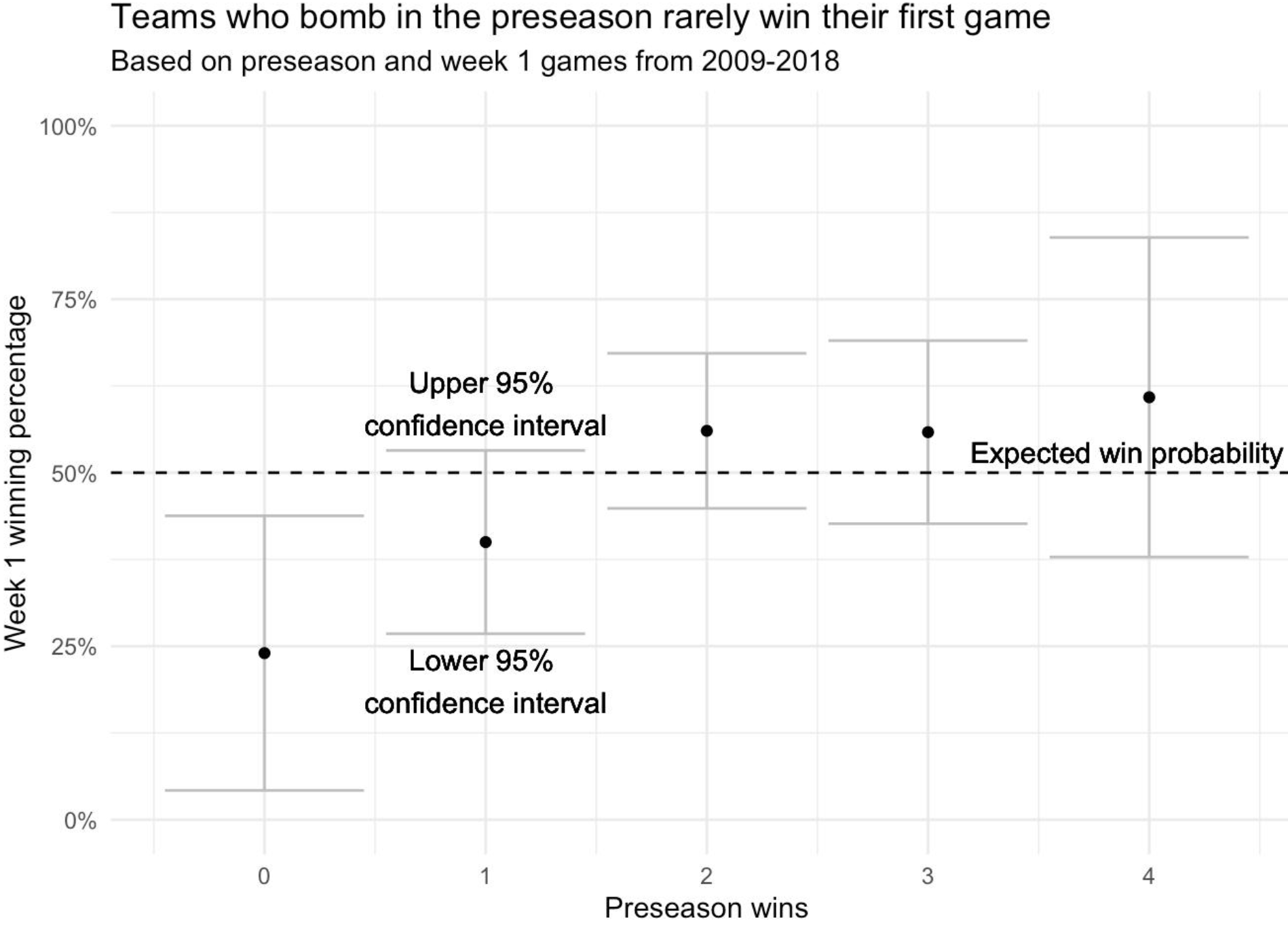
To see if there was any correlation I could find, I looked at week one outcomes. I figured if anything, good preseason results could indicate that a team was more prepared for their very first game of the season. To answer this question, I looked at the week one winning percentage for all teams by the number of games they won in the preseason. To account for the small sample size, I ran hypothesis tests for each outcome against the baseline week 1 win expected value of 50%.
week_1_plot_df <- all_game_data %>%
    mutate(winner = case_when(home_score > away_score ~ home_team,
                              away_score > home_score ~ away_team),
           loser = case_when(home_score > away_score ~ away_team,
                             away_score > home_score ~ home_team)) %>%
    filter((type == 'pre' | week == 1)) %>%
    count(season, type, winner, loser) %>%
    gather(outcome, team, c(winner, loser)) %>%
    group_by(team, season, type) %>%
    summarise(wins = sum(n[outcome == 'winner'])) %>%
    ungroup() %>%
    filter(!is.na(team)) %>%
    spread(type, wins) %>%
    group_by(pre) %>%
    filter(!is.na(reg)) %>%
    summarise(week_1_win_pct = mean(reg),
              n = n()) %>%
    ungroup()

plot_df <- map_df(1:nrow(week_1_plot_df), function(x) {
    this_row <- slice(week_1_plot_df, x)
    ttest <- prop.test(c(this_row$week_1_win_pct * this_row$n, .5 * sum(week_1_plot_df$n)),
                       c(this_row$n, sum(week_1_plot_df$n)))
    this_row %>%
        mutate(p_value = ttest$p.value,
               lower = .5 + ttest$conf.int[1],
               upper = .5 + ttest$conf.int[2])
})

ggplot(plot_df, aes(x = pre, y = week_1_win_pct)) +
    geom_errorbar(aes(ymax = upper, ymin = lower), color = 'grey') +
    geom_point() +
    theme_minimal() +
    geom_hline(yintercept = .5, linetype = 'dashed') +
    geom_text(x = 3.9, y = .53, label = 'Expected win probability') +
    geom_text(x = 1, y = .6, label = 'Upper 95% \nconfidence interval') +
    geom_text(x = 1, y = .2, label = 'Lower 95% \nconfidence interval') +
    scale_y_continuous(limits = c(0, 1), breaks = seq(0, 1, by = .25),
                       labels = function(x) percent(x, accuracy = 1)) +
    labs(x = 'Preseason wins',
         y = 'Week 1 winning percentage',
         title = 'Teams who bomb in the preseason rarely win their first game',
         subtitle = 'Based on preseason and week 1 games from 2009-2018')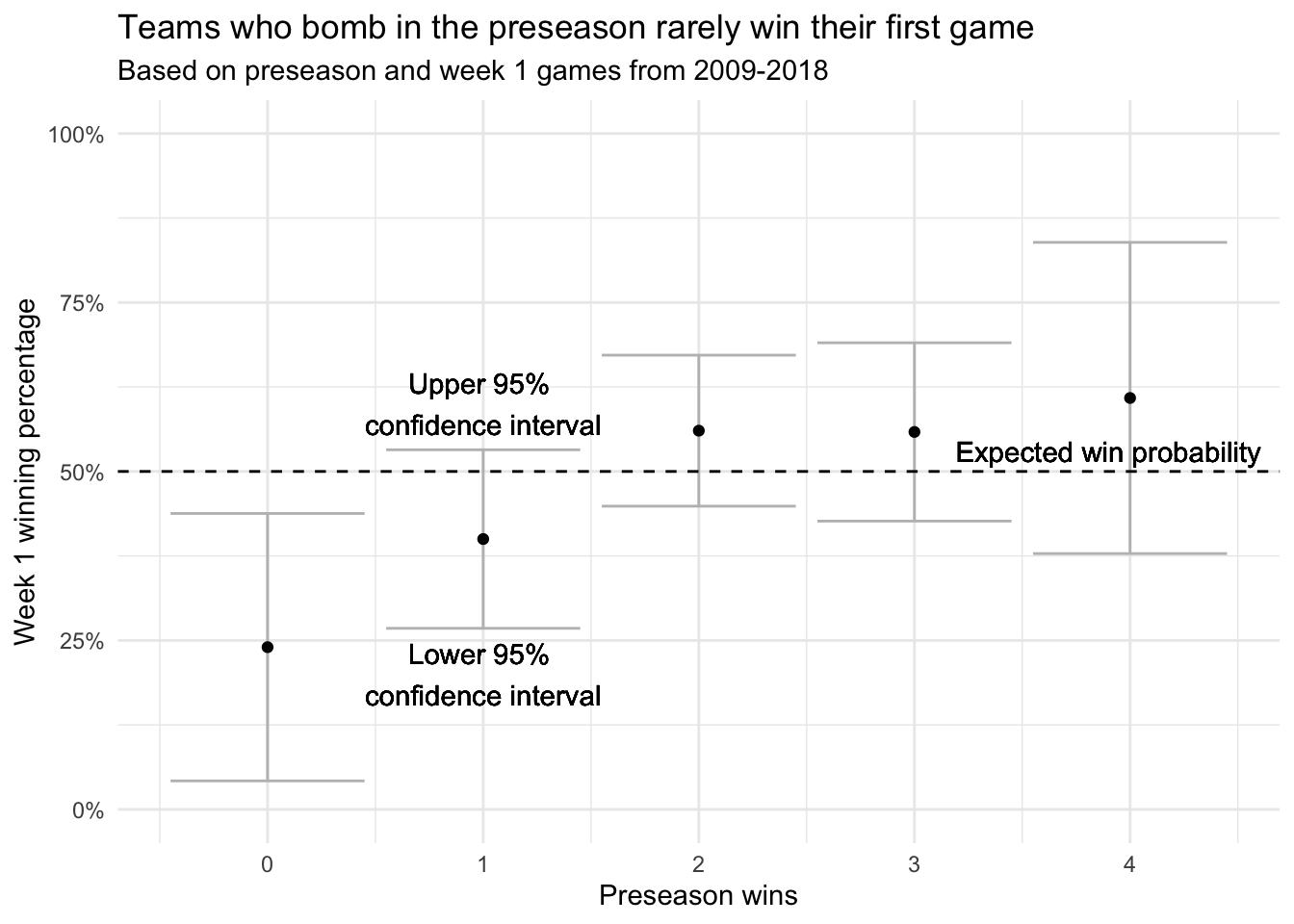
Here we do see a correlation! Teams who lose all four preseason games win their first game just 24% of the time, less than half the exepected value of 50%. That the upper 95% confidence interval is below 50% provides further evidence that a winless preseason lowers a team’s probability of winning their first game. Note that the small sample size (only 25 teams have lost every preseason game) widens the error bars and limits our ability to estimate the true probability with precision.
Interestingly, teams who win one preseason game do not lose their first game at a significantly higher rate than expected, which suggests that to be predictive of week 1, a team’s preseason performance needs to be truly disastrous.
On the other end, teams who win all four preseason games do not win their first game at a significantly higher rate than expected. This could mean that doing exceptionally well in the preseason isn’t as indicative of a well-prepared team as doing exceptionally poorly is indicative of being unprepared.
To verify this effect was unique to a team’s first game, I ran the same calculation on week 2.
week_2_plot_df <- all_game_data %>%
    mutate(winner = case_when(home_score > away_score ~ home_team,
                              away_score > home_score ~ away_team),
           loser = case_when(home_score > away_score ~ away_team,
                             away_score > home_score ~ home_team)) %>%
    filter(type == 'pre' | week == 2) %>%
    count(season, type, winner, loser) %>%
    gather(outcome, team, c(winner, loser)) %>%
    group_by(team, season, type) %>%
    summarise(wins = sum(n[outcome == 'winner'])) %>%
    ungroup() %>%
    filter(!is.na(team)) %>%
    spread(type, wins) %>%
    group_by(pre) %>%
    filter(!is.na(reg)) %>%
    summarise(week_2_win_pct = mean(reg),
              n = n()) %>%
    ungroup()

plot_df <- map_df(1:nrow(week_2_plot_df), function(x) {
        this_row <- slice(week_2_plot_df, x)
        ttest <- prop.test(c(this_row$week_2_win_pct * this_row$n, .5 * sum(week_2_plot_df$n)),
                           c(this_row$n, sum(week_2_plot_df$n)))
        this_row %>%
            mutate(p_value = ttest$p.value,
                   lower = .5 + ttest$conf.int[1],
                   upper = .5 + ttest$conf.int[2])
    })

ggplot(plot_df, aes(x = pre, y = week_2_win_pct)) +
    geom_errorbar(aes(ymax = upper, ymin = lower), color = 'grey') +
    geom_point() +
    theme_minimal() +
    geom_hline(yintercept = .5, linetype = 'dashed') +
    scale_y_continuous(limits = c(0, 1), breaks = seq(0, 1, by = .25),
                       labels = function(x) percent(x, accuracy = 1)) +
    labs(x = 'Preseason wins', y = 'Week 2 winning percentage',
         title = 'By week 2, the preseason effect goes away',
         subtitle = 'Based on preseason and week 2 games from 2009-2018')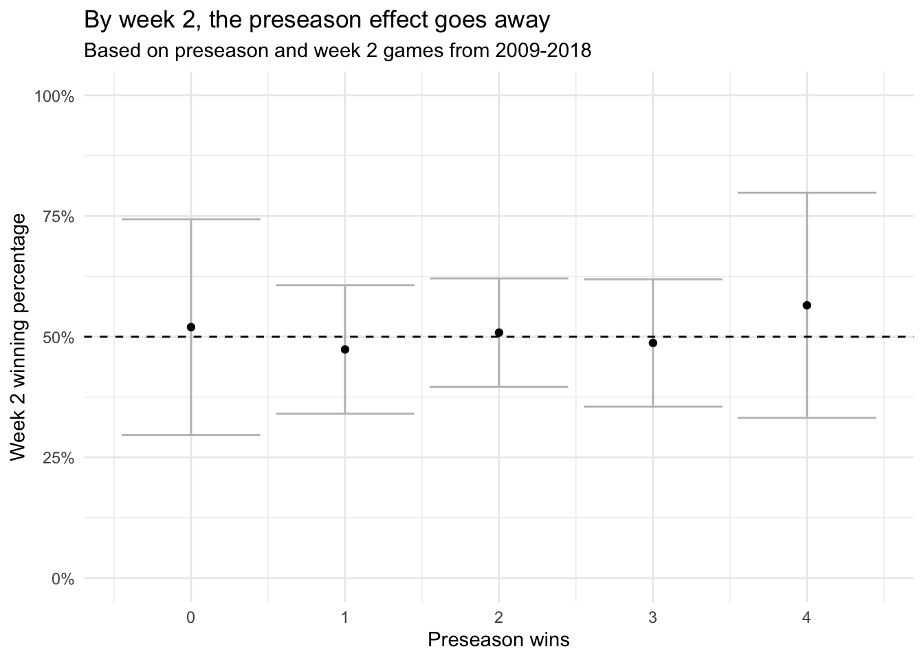
Here the winning percentages returned to the expected value of 50%, suggesting the preseason effect fades away after week 1.
In short, the preseason is, in fact, mostly useless for predicting the regular season - unless you totally bomb, in which case you’re somewhat less likely to win…but only in week 1. Still, I’d hesitate to put money on the Jaguars or the Lions (both 0-4 this preseason) next week.